GUI - Create Slices > Dr. Probe / Documentation / GUI / Sample

 

Creating sample data requires a sequence of 4 steps as indicated by the dialog text.

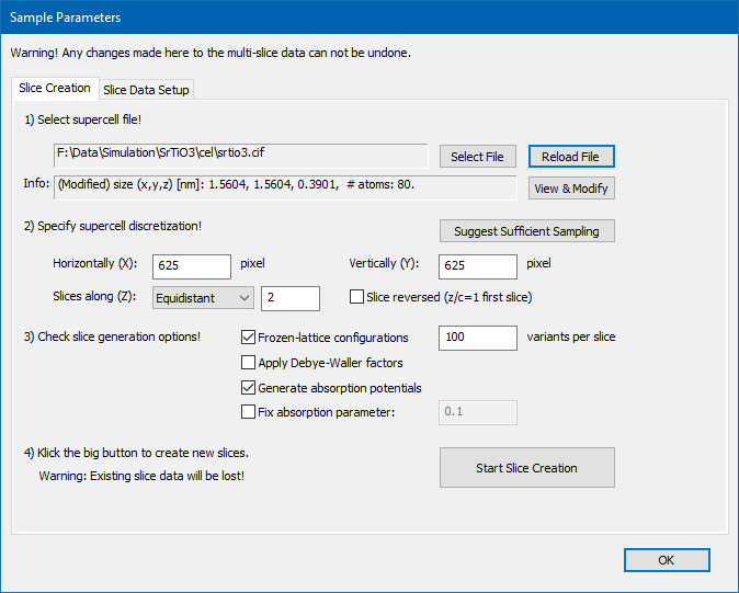
1. Load and modify an atomic structure model

Select a super-cell file containing the atomic structure model describing the sample. Choose either a CEL file or a CIF file for loading.

The selected file will be analyzed and loaded and information about the cell dimension and the number of atoms shown. The structure information from the displayed file name can be loaded again quickly by pressing the [Reload File] button.

It is recommended to always cross-check the loaded structure and in particular the B_iso parameters using the Structure modification dialog. Open this dialog by pressing the [View & Modify] button.

Dr. Probe requires an orthogonal super-cell as input for multislice calculations, i.e. a cell were all basis vectors are perpendicular to each other. If your structure has a non-orthogonal unit cell, the software will recognize this and deactivate the further processing of the structure model. Loaded structures can be orthogonalized and re-oriented externally by other programs such as CellMuncher or by pressing the [View & Modify] button.

2. Set the super-cell discretization

The phase grating data to be calculated is sampled in the x-y-plane using a user defined number of pixels. You may choose any number of pixels between 32 and 2048 for the horizontal N_x and the vertical sampling N_y. Higher pixel numbers result in a smaller sampling rate of the projected potentials and enable a calculation of larger scattering vectors. However, the calculation time increases with at least N · Log(N), where N = N_x · N_y is the total number of pixels. In order to keep the calculation time as short as possible you should also take care to use sampling numbers which are products of small prime factors: 2, 3, and 5.

Especially for simulations involving large angle scattering detection, e.g. high-angle annular dark-field STEM (HAADF), the number of pixels sampling the projected potentials may become quite large and need to be calculated in advance. Let s be the size of the super-cell along a certain direction in nanometers, then the sampling rate of the projected potentials is give by the quotient s / N_d, with N_d being the number of pixels used along this direction to sample the potentials. The same sampling rate and size is used later to calculate the propagation of the electron wave function through the object.

The sampling rate defines also the maximum spatial frequency g_max or the maximum diffraction vector q_max with

q_max / lambda ~ g_max = 1/2 · N_d / s,

where lambda is the electron wavelength.

Take into account, that a limiting aperture is applied during the multislice calculation in order to prevent artificial wrap-around of beams in Fourier space producing alias frequencies in the wave function. The aperture blocks all beams with

q > q_ap = 2/3 · q_max.

The maximum calculated diffraction angle is therefore

q_ap = 1/3 · N · lambda / s.

Consequently a minimum number of pixels N_min is required to calculate up to the maximum detection frequency q_det with

N_min = 3 q_det s / lambda.

The above directives are applied automatically when using the button [Suggest Sufficient Sampling]. This program function automatically sets the number of samples along x and y, taking into account current values of the size of the super-cell, the electron wavelength and the maximum angle of detection. The latter two parameters are taken from the current microscope parameter setup.

The slicing of the orthorhombic structure model along the main propagation direction z of the electron probe can be done in two different ways. A drop-down list lets you choose between a fully automatic scheme, which sets slice terminations at each atomic z coordinate in the structure if not closer to the previous termination than a few picometers. The edit box right next to the dropdown list is deactivated in this case, but displays the estimated number of slices for the current structure. The automatic slicing scheme can potentially create non-equidistant slices. The other option is the traditional equidistant slicing scheme. By choosing this scheme, you can set the number of slices N_z manually. A reasonable number of slices should correspond to the major (001) planes of the atomic structure. The function [Suggest Sufficient Sampling] tries to determine this number automatically from the distribution of atoms along the c-axis of the current super-cell.

The automatic slicing may fail or suggest very large numbers in cases of very complicated structures. It is recommended to check the proposed number of slices carefully. Very large number may lead to serious memory loading and extreme calculation times and are often not reasonable. As a rule of thumb, the average slice thickness (c / N_z) should not be significantly lower than 0.05 nm.

The equidistant sequence of slices begins by default at the fractional coordinate z/c = 0 of the input super-cell and ends with the last slice at the fractional coordinate z/c = 1. You may invert this sequence by checking the option "Slice reversed (z/c = 1 first slice)".

3. Select options for calculating scattering potentials

Additional options can be selected for the creation of the projected slice potentials. These options control in particular the simulation of thermal diffuse scattering and absorption.

For a frozen phonon calculation you should activate the option "Frozen-lattice configurations" and set the number of frozen lattice variants N_v appropriately. Partial atoms sharing one site by partial occupation will be moved coherently in frozen lattice configurations.

The number of slice variants N_v determines the number of frozen lattice states per slice, which are used to simulate random atomic displacements due to thermal vibrations. The mean atomic vibration amplitudes are calculated from the Debye-Waller parameters B in nm^2 as specified in the super-cell file. For a frozen-lattice calculation, the atomic potentials are displaced by a random distance from the respective equilibrium positions. A good range for the number of frozen-lattice variants N_v per slice is between 10 and 100, depending on the target object thickness, on the scan step size and on the periodicity of the object structure along the projection direction. In principle, N_v should be increased
- for smaller structure periods along the projection direction (smaller number of structure slices),
- for larger object thickness, and
- for smaller scan steps.

By activating the option "Apply Debye-Waller factors" the projected potentials dampened by a Gaussian Debye-Waller factor Exp[- 1/4 B g^2], where g denotes a spatial frequency. This can be a fast alternative for bright-field, low angle electron diffraction simulations with thin samples.

When using Debye-Waller factors, absorptive form factors as proposed by Weickenmeier and Kohl [Acta Cryst. A47 (1991) p. 590-597] are generated when checking the option "Generate absorption potentials". These potentials provide a fast way to simulate the intensity in the elastic channel for thin and weakly scattering samples.
When not using Debye-Waller factors, absorptive potentials will be generated to account for the electrons scattered to angles beyond the band-width limiting anti-alias aperture of the multislice calculation. The effect of this should be very small for sufficiently large grid sizes in frozen-lattice simulations.

Alternatively you may use the option to apply a "Fix absorption parameter", which effectively uses a certain fraction of the elastic scattering factor as absorptive form factor, as proposed by Hashimoto, Howie, and Whelan [Proc. R. Soc. London Ser. A, 269 (1962) p. 80-103]. For low-angle scattering calculations and medium Z materials a value around 0.1 is proposed. This is an empirical parameter often used to account for loss of intensity in bright-field and HRTEM simulations.

4. Start the calculation of object functions

Start the calculation process for phase gratings by clicking the button [Start Slice Creation]. Depending on the parameter setup, the calculation will require a significant amount of time and memory. You can approximate the required amount of memory M_slc in bytes by the formula

M_slc = 8 · N_x · N_y · N_z · N_v.

A popup dialog will appear with information on the slice generation progress with an option to abort the calculation. In case of aborting no slice data will be present afterwards, which means that previously existing slice data is lost.

After a successful calculation, new transmission functions are stored in memory and listed in the second page of the dialog for stacking them to a thick sample.

 

Last update: June 14, 2019    contact    disclaimer(de)