
|
Dr. Probe - frozen-lattice variation procedure |
Thermal atom vibrations have a significant effect in electron diffraction since they represent a deviation of the atomic object structure from the ideal symmetry of a crystal. When aiming for a quantitative evaluation of electron diffraction experiments by comparisons to simulations, the simulations have to consider the effects caused by thermal lattice distortions, which are frequently addressed as thermal diffuse scattering (TDS). The main difficulty for the incorporation of the related effects is that the approximations made to speed up electron diffraction calculations, be it by means of Bloch-waves, or by the multislice algorithm, assume an object with fix atom positions.
One can distinguish between two main routes for the consideration of TDS for the calculation of the elastic electron diffraction:
- Modification of the object scattering potential by Debye-Waller factors (DWF), and
- Averaging over repeated calculations using different frozen states of the crystal lattice (frozen lattice / frozen phonon).
The first route is a quasi-coherent approach, where, the atomic scattering factors are
convoluted by a Gaussian function approximating the distribution of atomic displacements.
The elastic electron diffraction is then calculated using the modified potentials, effectively
reducing the structure factors due to the deviations from the ideal crystal structure symmetry.
This approximation disregards any type of incoherent and diffuse scattering power.
The respective loss in the inelastic scattering channel is
usually registered by an absorptive form factor. For thin samples is also
possible to include the contribution of TDS in such a calculation [3].
The main drawback of the application of DWFs is that the large angle scattering, as recorded by
a high-angle annular dark-field (HAADF) detector, is massively compromised. Nevertheless, the
application of DWFs is the most efficient approach for the calculation of bright field electron
diffraction and is very frequently used for the calculation of coherent TEM images.
The second route provides a more realistic simulation of the electron diffraction also to larger scattering angles. The frozen lattice approximation is based on the assumption that each electron interacts with a specific static scattering potential. This assumption is in so far justified, since the velocity of the incident electrons, which is usually around one half of the speed of light for medium voltage electron microscopes (100 - 300 kV), is by several orders of magnitude larger than the speed of atoms due to thermal vibrations. In this view, each electron is scattered by a different frozen state of the lattice. The detected signal, to which up to several thousands of scattered electrons contribute, registers thus information from a large amount of different frozen lattice sates. Depending on the available data on the thermal vibration of the investigated crystal, an explicit phonon dispersion can be considered (frozen phonon approximation). Without specific information about the excitation of vibrational modes, usually incoherent atom vibrations are assumed (frozen lattice approximation). In both scenarios, usually a repeated computation of the electron diffraction is required, which amounts to a significant computation time when the system size is large, such as for large angle scattering calculations.
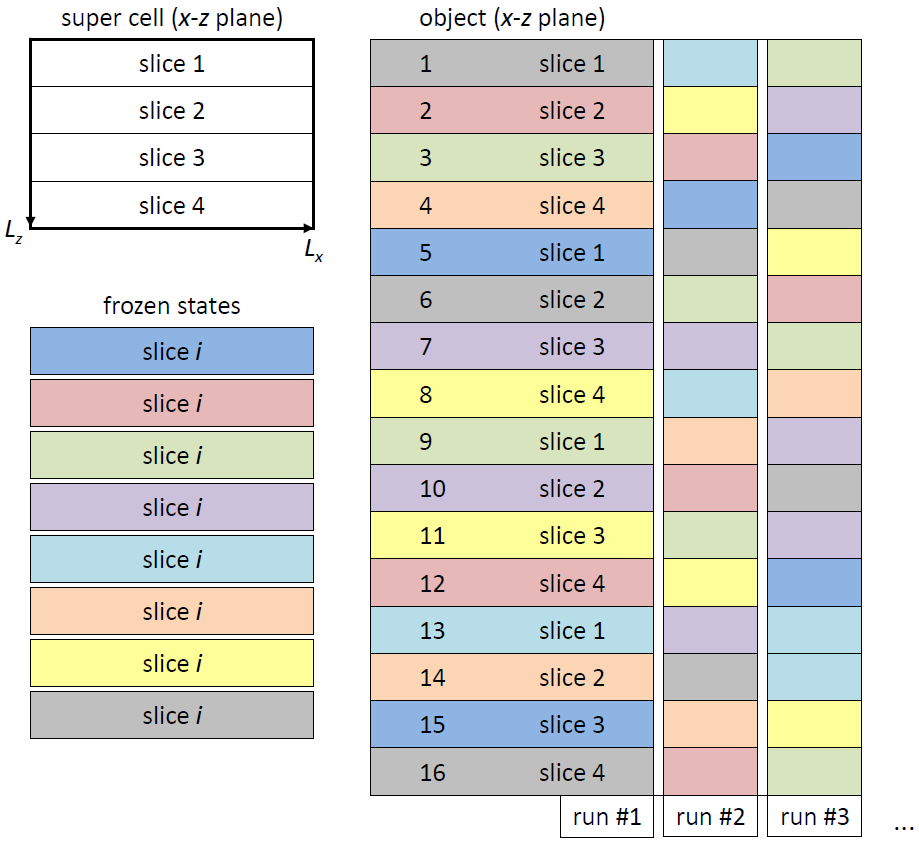
A time-efficient implementation of the multislice algorithm is applied by Dr. Probe. The implementation allows the simulation of thermal diffuse scattering using the frozen lattice approach. A set of M frozen lattice states is pre-calculated for each of the N object structure slices. The object slices are chosen as thin as possible containing preferably only one atomic plane. Projected potentials are calculated for all frozen states including random atom displacements to represent thermal atom vibrations. During one run of the multislice calculation one of the M pre-calculated frozen states of the current slice is selected randomly from the respective set of M states and applied to the current wave function in form of a phase grating. A random permutation of the pre-calculated frozen states is produced by repeated application of this random selection scheme over the whole sample thickness as illustrated by the figure below.
By this way one obtains free control over the number of frozen states applied to a scan pixel during run-time without additional calculation effort. The procedure allows for example to adapt the number of averaged frozen states locally depending on the local signal variation and thereby to optimize the total calculation time in conjunction with an improved simulation precision. A fast run-time variation of frozen states requires a previous loading of all pre-calculated frozen states (phase-grating slices) into the computer working memory. However, a large number of phase-grating pixels and frozen lattice states can be handled with commercially available computers supporting more than 4 Gigabytes working memory.
A minimum calculation time for a scan image is obtained by using only
one random permutation of frozen slice states per scan pixel. As expected,
this approach leads to a strong variation of the detected intensity per scan pixel.
The intensity variation from pixel to pixel is visible in the upper row of the
below figure, showing images composed of 40 x 40 scan pixels per projected
SrTiO3 [100] unit cell. For this simulation example, only one
frozen lattice permutation of the object consisting of 25 unit cell periods (50 slices)
was contributing to each pixel. However, the individual scan image pixels
where calculated with different combinations of frozen lattice states made up
from M = 50 pre-calculated frozen states for each of the two super cell slices.
A subsequent convolution of the images with an effective source profile is required
to obtain qualitatively and quantitatively correct images [4]. The images of the lower
row in the figure below are obtained by convolution of the respective upper row images
by a Gaussian source profile of 0.5 A 1/e-half-width. The convoluted images appear
smooth and represent also an average over frozen states applied to neighbor pixels
within the effective source radius (convolution radius).
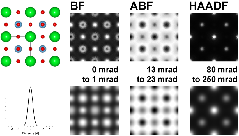
Model of 2x2 unit cells of SrTiO3 in [100] projection (size 7.812 A2) with Sr at the unit cell corners, Ti in the center and O at the faces. Exemplary simulated aberration-free bright-field (BF), annular bright-field (ABF), and high-angle annular dark-field (HAADF) images for 300 kV electrons, 25 mrad illumination half-angle, and 10 nm object thickness using one frozen lattice permutation per pixel. Detection angles are noted next to the respective images. The images of the top row are obtained before convolution with the effective source profile, the lower row shows the same images after convolution. The applied Gaussian source profile is displayed below the projected structure model and scaled to the size of the images.
This a-posteriori averaging of frozen states is possible due to a sufficiently small simulation scan step. In the present example, the scan step is approximately 10 pm per pixel, which is close to experimental scan steps frequently applied in high-resolution STEM. A sufficiently small scan step for a-posteriori frozen state averaging depends on the number of pixels per intensity peak in HAADF images before convolution and on the number of pixels within the effective source area for BF and ABF images.
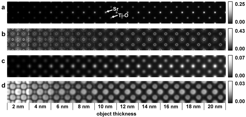
Series of simulated HAADF images illustrating the effective frozen-lattice averaging by a-posteriori source convolution of STEM images considering the same example as used in the above images. The images (a) and (c) show the average HAADF intensity of 90 statistically independent calculations relative to the incident probe intensity. Images (b) and (d) depict the standard deviation due to frozen-lattice variations of the 90 calculations relative to the average intensities of (a) and (c) respectively. The upper two image series are obtained before source-profile convolution, whereas the lower image series are obtained with convoluted images. Respective white-level scales are noted to the right, and the object thickness of the 2x2 unit cell patches is denoted below image (d).
Results of statistical evaluations from 90 independent calculations show a significant decrease of the pixel intensity variation after source profile convolution from approximately 40% down to 3% of the pixel mean value (see figure above). This precision level is sufficiently small for a comparison of simulation and experiment especially, when analyzing integrated column intensities. In conclusion, the consideration of just one frozen state per pixel is sufficient to obtain quantitatively meaningful simulation data when using realistic scan steps and subsequent source profile convolution.
References
- J.M. Cowley and A.F. Moodie, Acta. Cryst. 10 (1957) p. 609.
- R.F. Loane, P. Xu, and J. Silcox, Acta Cryst. A 47 (1991) p. 267.
- A. Rosenauer, M. Schowalter, J.T. Titantah, D. Lamoen, Ultramicroscopy 108 (2008) p. 1504.
- C. Dwyer, R. Erni, and J. Etheridge, Ultramicroscopy 110 (2010) p. 952.
Last update: Oct 16, 2023 contact disclaimer(de)